Calculations and Technical Explanations for Validation Metrics

Overview of the Evaluation Metrics involved:

Accuracy Score Calculation:

• Accuracy is one metric for evaluating classification models. It is the fraction of predictions that the classification model made correctly. (Reference: Multivariate Statistical Machine Learning Methods for Genomic Prediction, Page 111, Section 4.2. https://library.oapen.org/bitstream/handle/20.500.12657/52837/978-3-030-89010-0.pdf?sequence=1)

(1) The calculated value can be seen to be same as on the platform:

Using Formula

total_predictions = len(Predictions_np)
correct_predictions = 0
for i,j in zip(GroundTruths_np, Predictions_np):
    if i == j:
        correct_predictions = correct_predictions + 1
        
Acc = correct_predictions/total_predictions
print("Accuracy using Formula:", '\033[1m' ,round(Acc,4), '\033[0m')

Accuracy using Formula:  0.9222 

Using Library

from sklearn.metrics import accuracy_score

Acc = accuracy_score(GroundTruths_np, Predictions_np)
print("Accuracy using Library:", '\033[1m' ,round(Acc,4), '\033[0m')

Accuracy using Library:  0.9222 

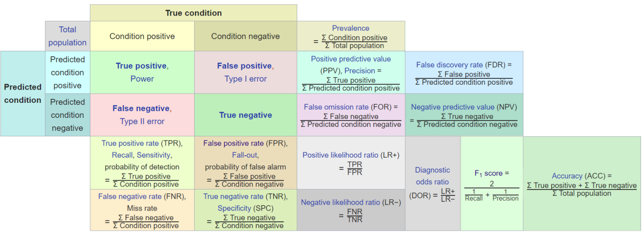
TP, TN, FP, FN:

• True Positive (TP): we predict a label of 1 (positive), and the true label is 1.
• True Negative (TN): we predict a label of 0 (negative), and the true label is 0.
• False Positive (FP): we predict a label of 1 (positive), but the true label is 0.
• False Negative (FN): we predict a label of 0 (negative), but the true label is 1.

from sklearn.metrics import confusion_matrix
TN1, FP1, FN1, TP1 = confusion_matrix(GroundTruths_np, Predictions_np).ravel()
FPR1 = FP1 / (FP1+TN1)

print("For 'Pneumonia':" , "\n")
print("True Positives:", '\033[1m' ,TP1, '\033[0m')
print("True Negatives:", '\033[1m' ,TN1, '\033[0m')    
print("False Positives:", '\033[1m' ,FP1, '\033[0m')
print("False Negatives:", '\033[1m' ,FN1, '\033[0m', "\n", "\n")

TP2 = np.sum(np.logical_and(Predictions_np == 0, GroundTruths_np == 0))
TN2 = np.sum(np.logical_and(Predictions_np == 1, GroundTruths_np == 1))
FP2 = np.sum(np.logical_and(Predictions_np == 0, GroundTruths_np == 1))
FN2 = np.sum(np.logical_and(Predictions_np == 1, GroundTruths_np == 0))
FPR2 = FP2 / (FP2+TN2)

print("For 'Normal':", "\n")
print("True Positives:", '\033[1m' ,TP2, '\033[0m')
print("True Negatives:", '\033[1m' ,TN2, '\033[0m')    
print("False Positives:", '\033[1m' ,FP2, '\033[0m')
print("False Negatives:", '\033[1m' ,FN2, '\033[0m')

For 'Pneumonia': 
    
True Positives:  3702 
True Negatives:  14763 
False Positives:  364 
False Negatives:  1194 
     
    
For 'Normal': 
    
True Positives:  14763 
True Negatives:  3702 
False Positives:  1194 
False Negatives:  364 

Micro F1 Calculation:

• F1 score is an error metric which measures model performance by calculating the harmonic mean of precision and recall for the minority positive class.
• Micro F1 calculates a global average F1 score by counting the sums of the True Positives (TP), False Negatives (FN), and False Positives (FP).(Reference: https://riskcue.id/uploads/ebook/20210920085146-2021-09-20ebook085121.pdf)

(2) The calculated value can be seen to be same as on the platform:

Using Formula

TP = TP1+TP2
FP = FP1+FP2
TN = TN1+TN2
FN = FN1+FN2
Micro_F1 = TP / (TP + 0.5*(FP+FN))
print("Micro F1:", '\033[1m' ,round(Micro_F1,4), '\033[0m')

Micro F1:  0.9222 

Using Library

from sklearn.metrics import f1_score
Micro_F1 = f1_score(GroundTruths_np, Predictions_np, average='micro')
print("Micro F1:", '\033[1m' ,round(Micro_F1,4), '\033[0m')

Micro F1:  0.9222 

Macro F1 Calculation:

• Macro F1 score is the unweighted mean of the F1 scores calculated per class. It is the simplest aggregation for F1 score. It is calculated using the arithmetic mean (aka unweighted mean) of F1 scores of both classes. (Reference: https://riskcue.id/uploads/ebook/20210920085146-2021-09-20ebook085121.pdf)

(3) The calculated value can be seen to be same as on the platform:

Using Formula

Precision1 = TP1 / (TP1 + FP1)
Precision2 = TP2 / (TP2 + FP2)
Recall1 = TP1 / (TP1 + FN1)
Recall2 = TP2 / (TP2 + FN2)
F1_1 = (2 * Precision1 * Recall1) / (Precision1 + Recall1)
F1_2 = (2 * Precision2 * Recall2) / (Precision2 + Recall2)
Macro_F1 = (F1_1 + F1_2) / 2
print("Macro F1:", '\033[1m' ,round(Macro_F1,3), '\033[0m')

Macro F1:  0.888 

Using Library

from sklearn.metrics import f1_score

Macro_F1 = f1_score(GroundTruths_np, Predictions_np, average='macro')
print("Macro F1:", '\033[1m' ,round(Macro_F1,3), '\033[0m')

Macro F1:  0.888 

AUC Score:

• AUC stands for "Area under the ROC Curve." That is, AUC measures the entire two-dimensional area underneath the entire ROC.
• AUC ranges in value from 0 to 1. A model whose predictions are 100% wrong has an AUC of 0.0; one whose predictions are 100% correct has an AUC of 1.0. (Reference: https://developers.google.com/machine-learning/crash-course/classification/roc-and-auc)

(4) The calculated value can be seen to be same as on the platform:

Using Formula + Library

from sklearn.metrics import roc_curve
from sklearn.metrics import auc
GT_binarized= np.array([[1,0] if l==1 else [0,1] for l in GroundTruths_np])
Probs = np.column_stack((Class_1_Confidence_np,Class_2_Confidence_np))
fpr = {}
tpr = {}
roc_auc = dict()
classes = [0,1]
n_classes = len(classes)
for i in range(n_classes):    
    fpr[i], tpr[i], _ = roc_curve(GT_binarized[:,i], Probs[:,i])
    roc_auc[i] = auc(fpr[i], tpr[i])

all_fpr = np.unique(np.concatenate([fpr[i] for i in range(n_classes)]))
mean_tpr = np.zeros_like(all_fpr)
for i in range(n_classes):
    mean_tpr += np.interp(all_fpr, fpr[i], tpr[i])
     
mean_tpr /= n_classes
fpr["macro"] = all_fpr
tpr["macro"] = mean_tpr
roc_auc["macro"] = auc(fpr["macro"], tpr["macro"])
roc1 = roc_auc["macro"]

print("AUC Score:", '\033[1m' ,round(roc1,4), '\033[0m')

AUC Score:  0.9666 

Positive Predictive Value (PPV) (Precision) Calculation:

• Precision is defined as the ratio of correctly classified positive samples (True Positive) to a total number of classified positive samples (either correctly or incorrectly). (Reference: Multivariate Statistical Machine Learning Methods for Genomic Prediction, Page 132, Section 4.5.2. https://library.oapen.org/bitstream/handle/20.500.12657/52837/978-3-030-89010-0.pdf?sequence=1)

(5) The calculated value can be seen to be same as on the platform:

Using Formula

Precision1 = TP1 / (TP1 + FP1)
Precision2 = TP2 / (TP2 + FP2)
Precision = (Precision1+Precision2) / 2
print("Precision (PPV):", '\033[1m' ,round(Precision,4), '\033[0m')

Precision (PPV):  0.9178 

Using Library

from sklearn.metrics import precision_score
PPV = precision_score(GroundTruths_np, Predictions_np, average='macro')
print("Precision (PPV):", '\033[1m' ,round(PPV,4), '\033[0m')

Precision (PPV):  0.9178 

Negative Predictive Value (NPV) (Sensitivity) Calculation:

• In Binary classification, the NPV (recall) of the positive class is also known as “sensitivity”. (Reference: Multivariate Statistical Machine Learning Methods for Genomic Prediction, Page 132, Section 4.5.2. https://library.oapen.org/bitstream/handle/20.500.12657/52837/978-3-030-89010-0.pdf?sequence=1)

(6) The calculated value can be seen to be same as on the platform:

Using Formula

NPV = (Recall1 + Recall2)/2
print("NPV (Sensitivity):",'\033[1m' ,round(NPV,4), '\033[0m')

NPV (Sensitivity):  0.866 

Using Library

from sklearn.metrics import recall_score
Sensitivity = NPV = recall_score(GroundTruths_np, Predictions_np, average='macro')
print("Recall (NPV):", '\033[1m' ,round(NPV,4), '\033[0m')

Recall (NPV):  0.866 

Specificity Calculation:

• In Binary classification, the recall of the negative class is also known as “specificity”. (Reference: Multivariate Statistical Machine Learning Methods for Genomic Prediction, Page 132, Section 4.5.2. https://library.oapen.org/bitstream/handle/20.500.12657/52837/978-3-030-89010-0.pdf?sequence=1)

(7) The calculated value can be seen to be same as on the platform:

Using Formula

Specificity = (Recall1+Recall2)/2
print("Specificity:", '\033[1m' ,round(Specificity,4), '\033[0m')

    Specificity:  0.866 

Matthews Correlation Coefficient Calculation:

• Reference: Multivariate Statistical Machine Learning Methods for Genomic Prediction, Page 136, Line 1. (https://library.oapen.org/bitstream/handle/20.500.12657/52837/978-3-030-89010-0.pdf?sequence=1)

(8) The calculated value can be seen to be same as on the platform:

Using Formula

MCC = ((TP1*TN1)-(FP1*FN1))/(math.sqrt((TP1+FP1)*(TP1+FN1)*(TN1+FP1)*(TN1+FN1)))  
print("Mathews C.C:", '\033[1m' ,round(MCC,4), '\033[0m')

Mathews C.C:  0.7821 

Using Library

from sklearn.metrics import matthews_corrcoef
MCC = matthews_corrcoef(GroundTruths_np, Predictions_np)
print("Mathews C.C:", '\033[1m' ,round(MCC,4), '\033[0m')

Mathews C.C:  0.7821

Table, Graphs and Charts:

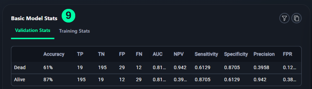
Basic Model Stats

• Table shows the status of the model with respect to every class of data on which the model is trained.

(9) Results from the Snapshot of the platform can be compared with the documented results here:

from tabulate import tabulate
n = 0
p = 0
t1=0
t2=0
for i in range(np.size(GroundTruths_np)):
    if GroundTruths_np[i] == 0:
        t1 = t1+1
        if GroundTruths_np[i]==Predictions_np[i]:
            n = n+1
                
    elif GroundTruths_np[i] == 1:
        t2 = t2+1
        if GroundTruths_np[i]==Predictions_np[i]:
            p = p+1
Acc2 = n/t1
Acc1 = p/t2

table = [['','Accuracy', 'TP', 'TN', 'FP', 'FN', 'Sensitivity', 'Specificity', 'Precision', 'FPR'], 
["Normal",f'{round(Acc2*100)}'+'%',TP2,TN2,FP2,FN2,round(Recall2,4),
round(Recall1,4),round(Precision2,4),round(FPR2,4)], 
["Pneumonia",f'{round(Acc1*100)}'+'%',TP1,TN1,FP1,FN1,round(Recall1,4),
round(Recall2,4),round(Precision1,4),round(FPR1,4)]]

print(tabulate(table, headers='firstrow', tablefmt='fancy_grid')) 

    ╒═══════════╤════════════╤═══════╤═══════╤══════╤══════╤═══════════════╤═══════════════╤═════════════╤════════╕
    │           │ Accuracy   │    TP │    TN │   FP │   FN │   Sensitivity │   Specificity │   Precision │    FPR │
    ╞═══════════╪════════════╪═══════╪═══════╪══════╪══════╪═══════════════╪═══════════════╪═════════════╪════════╡
    │ Normal    │ 98%        │ 14763 │  3702 │ 1194 │  364 │        0.9759 │        0.7561 │      0.9252 │ 0.2439 │
    ├───────────┼────────────┼───────┼───────┼──────┼──────┼───────────────┼───────────────┼─────────────┼────────┤
    │ Pneumonia │ 76%        │  3702 │ 14763 │  364 │ 1194 │        0.7561 │        0.9759 │      0.9105 │ 0.0241 │
    ╘═══════════╧════════════╧═══════╧═══════╧══════╧══════╧═══════════════╧═══════════════╧═════════════╧════════╛

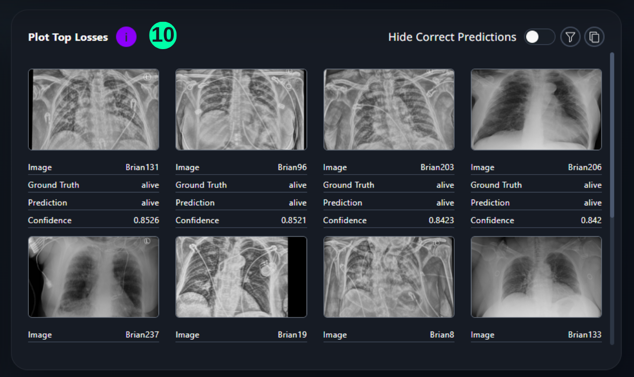
Top Losses

• This section shows the images which have the highest confidence score with an incorrect prediction, in a descending order.

(10) Results from the Snapshot of the platform can be compared with the documented results here.

Overall_df
new_df = Overall_df
new_df['Top_Loss']=np.where((new_df['Ground_Truth'] != new_df['Prediction']), new_df['Class_1_Confidence'], np.nan)
t_losses_df = pd.DataFrame().assign(Image_ID = new_df['Image_ID'], Confidence = new_df['Top_Loss'], 
                                    Ground_Truth = new_df['Ground_Truth'], Prediction = new_df['Prediction'])
t_losses_df = t_losses_df.dropna()
t_losses_df = t_losses_df.sort_values(by='Confidence', ascending = False, ignore_index=True)
print(t_losses_df.head(5))

table1 = [['Image',t_losses_df['Image_ID'][0],t_losses_df['Image_ID'][1],
t_losses_df['Image_ID'][2],t_losses_df['Image_ID'][3],t_losses_df['Image_ID'][4]], 
["Ground Truth",'Normal','Normal','Normal','Normal','Normal'],
['Prediction','Pneumonia','Pneumonia','Pneumonia','Pneumonia','Pneumonia'],
["Confidence",t_losses_df['Confidence'][0],t_losses_df['Confidence'][1],
t_losses_df['Confidence'][2],t_losses_df['Confidence'][3],t_losses_df['Confidence'][4]]]

print(tabulate(table1, headers='firstrow', tablefmt='fancy_grid'))

               Image_ID  Confidence  Ground_Truth  Prediction
    0     covid_image33       0.731             0           1
    1    covid_image161       0.731             0           1
    2    covid_image208       0.731             0           1
    3     covid_image72       0.731             0           1
    4  covid_image19384       0.731             0           1
    ╒══════════════╤═════════════════╤══════════════════╤══════════════════╤═════════════════╤════════════════════╕
    │ Image        │ covid_image33   │ covid_image161   │ covid_image208   │ covid_image72   │ covid_image19384   │
    ╞══════════════╪═════════════════╪══════════════════╪══════════════════╪═════════════════╪════════════════════╡
    │ Ground Truth │ Normal          │ Normal           │ Normal           │ Normal          │ Normal             │
    ├──────────────┼─────────────────┼──────────────────┼──────────────────┼─────────────────┼────────────────────┤
    │ Prediction   │ Pneumonia       │ Pneumonia        │ Pneumonia        │ Pneumonia       │ Pneumonia          │
    ├──────────────┼─────────────────┼──────────────────┼──────────────────┼─────────────────┼────────────────────┤
    │ Confidence   │ 0.731           │ 0.731            │ 0.731            │ 0.731           │ 0.731              │
    ╘══════════════╧═════════════════╧══════════════════╧══════════════════╧═════════════════╧════════════════════╛

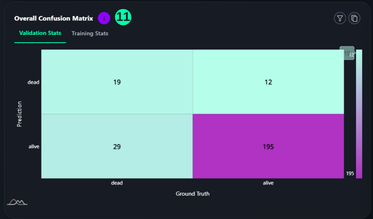
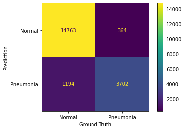
Overall Confusion Matrix

• A confusion matrix is a tabular summary of the number of correct and incorrect predictions made by a classification model. Its 4 sections show the TP, TN, FP, and FP counts. (Reference: Multivariate Statistical Machine Learning Methods for Genomic Prediction, Page 131, Section 4.5.2. https://library.oapen.org/bitstream/handle/20.500.12657/52837/978-3-030-89010-0.pdf?sequence=1)

(11) Results from the Snapshot of the platform can be compared with the documented results here:

from sklearn.metrics import confusion_matrix, ConfusionMatrixDisplay

cm = confusion_matrix(GroundTruths_np, Predictions_np)
cmd = ConfusionMatrixDisplay(cm, display_labels=['Normal','Pneumonia'])
cmd.plot()
cmd.ax_.set(xlabel='Ground Truth', ylabel='Prediction')

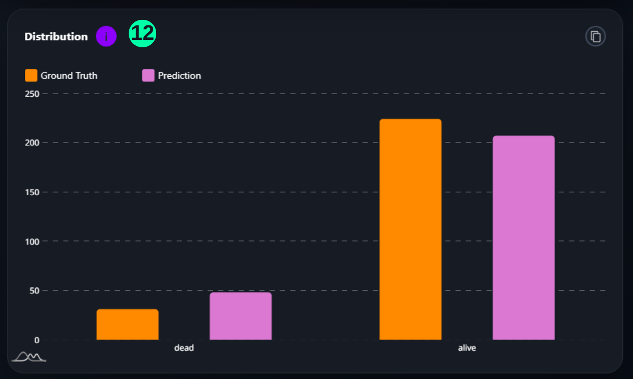
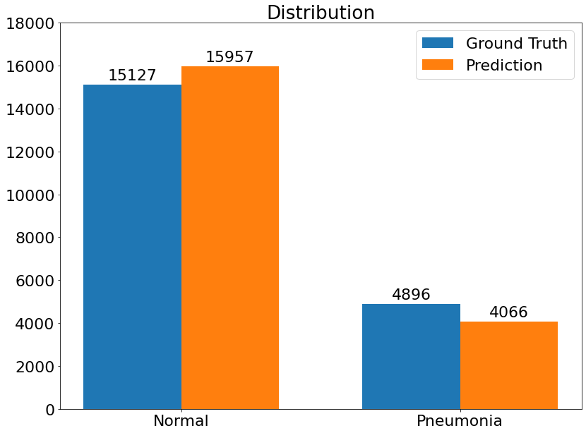
Distribution

• This is the Prediction Ground Truth Distribution, which visualizes the distibution of Ground Truth and Prediction number amongst both classes.

(12) Results from the Snapshot of the platform can be compared with the documented results here.

import matplotlib.pyplot as plt
plt.rcParams.update({'font.size': 22})
GT_N = 0
GT_Pn = 0
Pr_N = 0
Pr_Pn = 0

for i in GroundTruths_np:
    if i == 0:
        GT_N = GT_N + 1
    elif i == 1:
        GT_Pn = GT_Pn + 1
        
for i in Predictions_np:
    if i == 0:
        Pr_N = Pr_N + 1
    elif i == 1:
        Pr_Pn = Pr_Pn + 1

plt.rcParams["figure.figsize"] = (12,9)

labels = ['Normal', 'Pneumonia']
GT = [GT_N, GT_Pn]
PNeu = [Pr_N, Pr_Pn]

x = np.arange(len(labels))  # the label locations
width = 0.35  # the width of the bars

fig, ax = plt.subplots()
rects1 = ax.bar(x - width/2, GT, width, label='Ground Truth')
rects2 = ax.bar(x + width/2, PNeu, width, label='Prediction')

# Add some text for labels, title and custom x-axis tick labels, etc.
ax.set_title('Distribution')
ax.set_xticks(x, labels)
ax.legend()

ax.bar_label(rects1, padding=3)
ax.bar_label(rects2, padding=3)

fig.tight_layout()
plt.ylim([0, 18000]) 
plt.show()

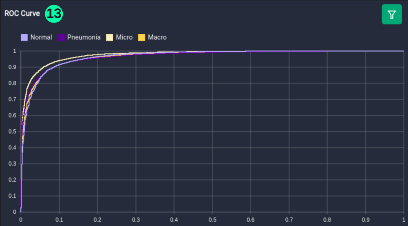
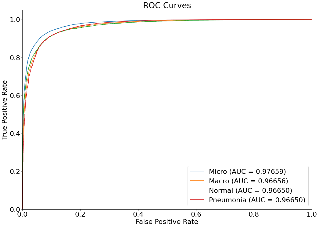
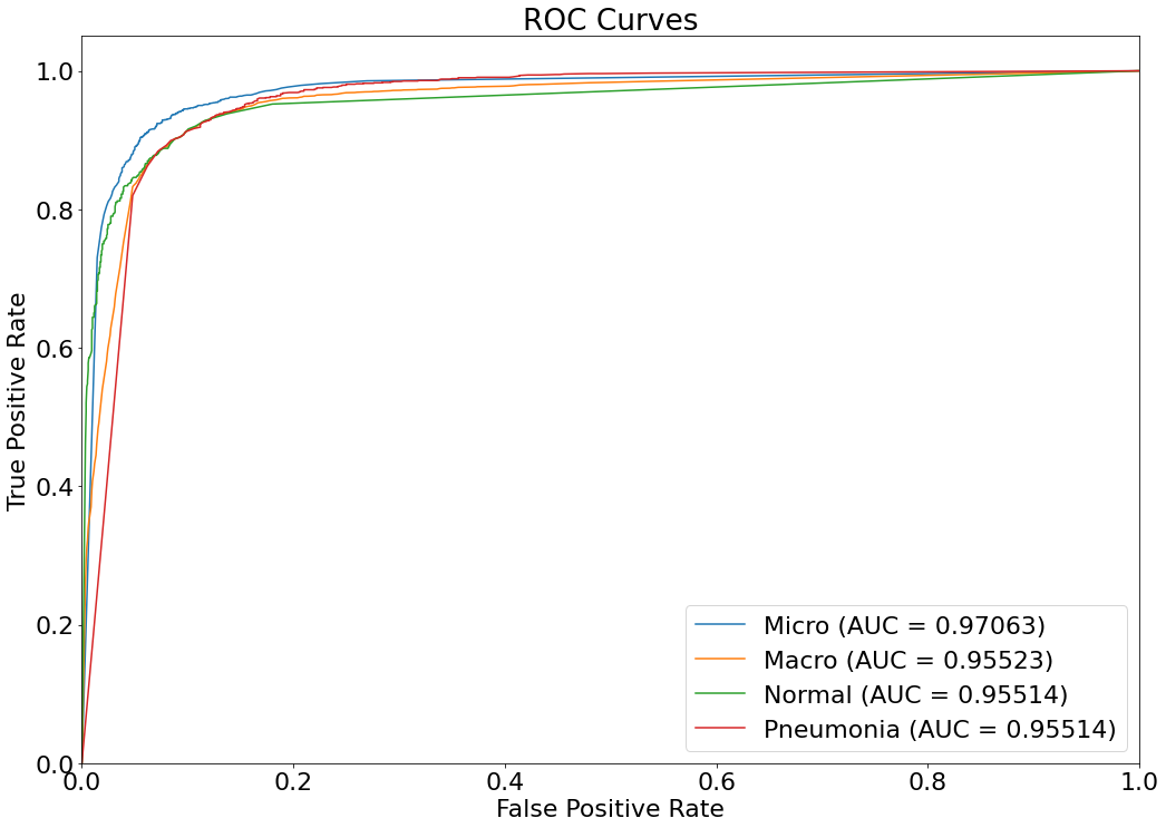
ROC Curve

• An ROC (Receiver Operating Characteristic) curve is a graph showing the performance of a classification model at all classification thresholds. This curve plots two parameters: True Positive Rate & False Positive Rate. (Reference: Multivariate Statistical Machine Learning Methods for Genomic Prediction, Page 131, Section 4.5.2. https://library.oapen.org/bitstream/handle/20.500.12657/52837/978-3-030-89010-0.pdf?sequence=1)

(13) Results from the Snapshot of the platform can be compared with the documented results here:

from sklearn.metrics import roc_curve
from sklearn.metrics import auc

GT_binarized= np.array([[1,0] if l==1 else [0,1] for l in GroundTruths_np])
Probs = np.column_stack((Class_1_Confidence_np,Class_2_Confidence_np))

fpr = {}
tpr = {}
thresh ={}
roc_auc = dict()

classes = [0,1]
n_classes = len(classes)

for i in range(n_classes):    
    fpr[i], tpr[i], _ = roc_curve(GT_binarized[:,i], Probs[:,i])
    roc_auc[i] = auc(fpr[i], tpr[i])


all_fpr = np.unique(np.concatenate([fpr[i] for i in range(n_classes)]))
mean_tpr = np.zeros_like(all_fpr)
for i in range(n_classes):
    mean_tpr += np.interp(all_fpr, fpr[i], tpr[i])
    
mean_tpr /= n_classes
fpr["macro"] = all_fpr
tpr["macro"] = mean_tpr
roc_auc["macro"] = auc(fpr["macro"], tpr["macro"])

fpr["micro"], tpr["micro"], _ = roc_curve(GT_binarized.ravel(), Probs.ravel())
roc_auc["micro"] = auc(fpr["micro"], tpr["micro"])


# Plot ROC curve
plt.figure(figsize=(17, 12))
plt.plot(fpr["micro"], tpr["micro"],
         label='Micro (AUC = {0:0.5f})'
               ''.format(roc_auc["micro"]))

plt.plot(fpr["macro"], tpr["macro"],
         label='Macro (AUC = {0:0.5f})'
               ''.format(roc_auc["macro"]))

labels = ['Normal', 'Pneumonia']
for i in range(n_classes):
    plt.plot(fpr[i], tpr[i], label='{0} (AUC = {1:0.5f})'
                                   ''.format(labels[i], roc_auc[i]))

plt.xlim([0.0, 1.0])
plt.ylim([0.0, 1.05])
plt.xlabel('False Positive Rate')
plt.ylabel('True Positive Rate')
plt.title('ROC Curves')
plt.legend(loc="lower right")
plt.show()

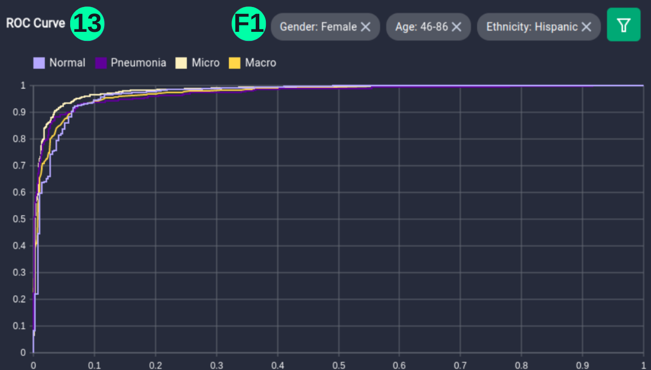
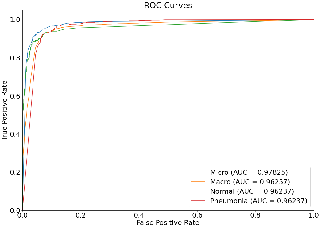
- The dataset and predictions can be filtered with metadata elements using the filter button, involving Age, Gender, and Ethnicity of the person, and ROC curves can be visualized for this setting.

(13)(F1) Filters and the resulting graph can be seen from the Snapshot of the platform and compared with the documented results here:

Filtered_DF_1 = Overall_df[(Overall_df['Age'].between(46, 86) & Overall_df['Ethnicity'].isin(['Hispanic'])) & 
          Overall_df['Gender'].isin(['Female'])] 

GT_F1_np = (pd.DataFrame().assign(Ground_Truth=Filtered_DF_1['Ground_Truth'])).to_numpy()
C1_F1_np = (pd.DataFrame().assign(Class_1_Confidence=Filtered_DF_1['Class_1_Confidence'])).to_numpy()
C2_F1_np = (pd.DataFrame().assign(Class_0_Confidence=Filtered_DF_1['Class_0_Confidence'])).to_numpy()


GT_F1_binarized= np.array([[1,0] if l==1 else [0,1] for l in GT_F1_np])
Probs_F1_np = np.column_stack((C1_F1_np,C2_F1_np))

fpr = {}
tpr = {}
thresh ={}
roc_auc = dict()

classes = [0,1]
n_classes = len(classes)

for i in range(n_classes):    
    fpr[i], tpr[i], _ = roc_curve(GT_F1_binarized[:,i], Probs_F1_np[:,i])
    roc_auc[i] = auc(fpr[i], tpr[i])


all_fpr = np.unique(np.concatenate([fpr[i] for i in range(n_classes)]))
mean_tpr = np.zeros_like(all_fpr)
for i in range(n_classes):
    mean_tpr += np.interp(all_fpr, fpr[i], tpr[i])
    
mean_tpr /= n_classes
fpr["macro"] = all_fpr
tpr["macro"] = mean_tpr
roc_auc["macro"] = auc(fpr["macro"], tpr["macro"])

fpr["micro"], tpr["micro"], _ = roc_curve(GT_F1_binarized.ravel(), Probs_F1_np.ravel())
roc_auc["micro"] = auc(fpr["micro"], tpr["micro"])
    

# Plot ROC curve
plt.figure(figsize=(17, 12))
plt.plot(fpr["micro"], tpr["micro"],
         label='Micro (AUC = {0:0.5f})'
               ''.format(roc_auc["micro"]))

plt.plot(fpr["macro"], tpr["macro"],
         label='Macro (AUC = {0:0.5f})'
               ''.format(roc_auc["macro"]))

labels = ['Normal', 'Pneumonia']
for i in range(n_classes):
    plt.plot(fpr[i], tpr[i], label='{0} (AUC = {1:0.5f})'
                                   ''.format(labels[i], roc_auc[i]))

plt.xlim([0.0, 1.0])
plt.ylim([0.0, 1.05])
plt.xlabel('False Positive Rate')
plt.ylabel('True Positive Rate')
plt.title('ROC Curves')
plt.legend(loc="lower right")
plt.show()

(13)(F2) Filters and the resulting graph can be seen from the Snapshot of the platform and compared with the documented results here:

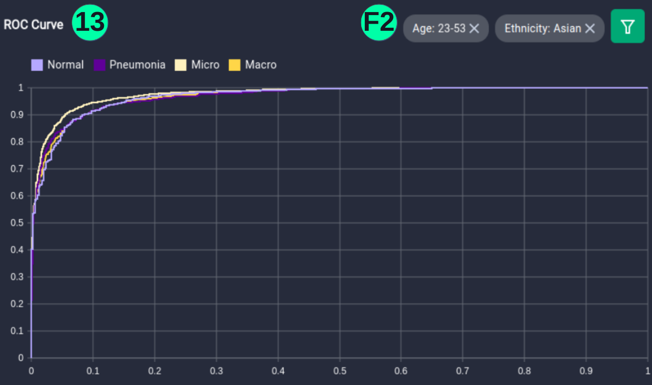
Filtered_DF_2 = Overall_df[(Overall_df['Age'].between(23, 53) & Overall_df['Ethnicity'].isin(['Asian']))] 


GT_F2_np = (pd.DataFrame().assign(Ground_Truth=Filtered_DF_2['Ground_Truth'])).to_numpy()
C1_F2_np = (pd.DataFrame().assign(Class_1_Confidence=Filtered_DF_2['Class_1_Confidence'])).to_numpy()
C2_F2_np = (pd.DataFrame().assign(Class_0_Confidence=Filtered_DF_2['Class_0_Confidence'])).to_numpy()


GT_F2_binarized= np.array([[1,0] if l==1 else [0,1] for l in GT_F2_np])
Probs_F2_np = np.column_stack((C1_F2_np,C2_F2_np))

fpr = {}
tpr = {}
thresh ={}
roc_auc = dict()

classes = [0,1]
n_classes = len(classes)

for i in range(n_classes):    
    fpr[i], tpr[i], _ = roc_curve(GT_F2_binarized[:,i], Probs_F2_np[:,i])
    roc_auc[i] = auc(fpr[i], tpr[i])


all_fpr = np.unique(np.concatenate([fpr[i] for i in range(n_classes)]))
mean_tpr = np.zeros_like(all_fpr)
for i in range(n_classes):
    mean_tpr += np.interp(all_fpr, fpr[i], tpr[i])
    
mean_tpr /= n_classes
fpr["macro"] = all_fpr
tpr["macro"] = mean_tpr
roc_auc["macro"] = auc(fpr["macro"], tpr["macro"])

fpr["micro"], tpr["micro"], _ = roc_curve(GT_F2_binarized.ravel(), Probs_F2_np.ravel())
roc_auc["micro"] = auc(fpr["micro"], tpr["micro"])
    

# Plot ROC curve
plt.figure(figsize=(17, 12))
plt.plot(fpr["micro"], tpr["micro"],
         label='Micro (AUC = {0:0.5f})'
               ''.format(roc_auc["micro"]))

plt.plot(fpr["macro"], tpr["macro"],
         label='Macro (AUC = {0:0.5f})'
               ''.format(roc_auc["macro"]))

labels = ['Normal', 'Pneumonia']
for i in range(n_classes):
    plt.plot(fpr[i], tpr[i], label='{0} (AUC = {1:0.5f})'
                                   ''.format(labels[i], roc_auc[i]))

plt.xlim([0.0, 1.0])
plt.ylim([0.0, 1.05])
plt.xlabel('False Positive Rate')
plt.ylabel('True Positive Rate')
plt.title('ROC Curves')
plt.legend(loc="lower right")
plt.show()

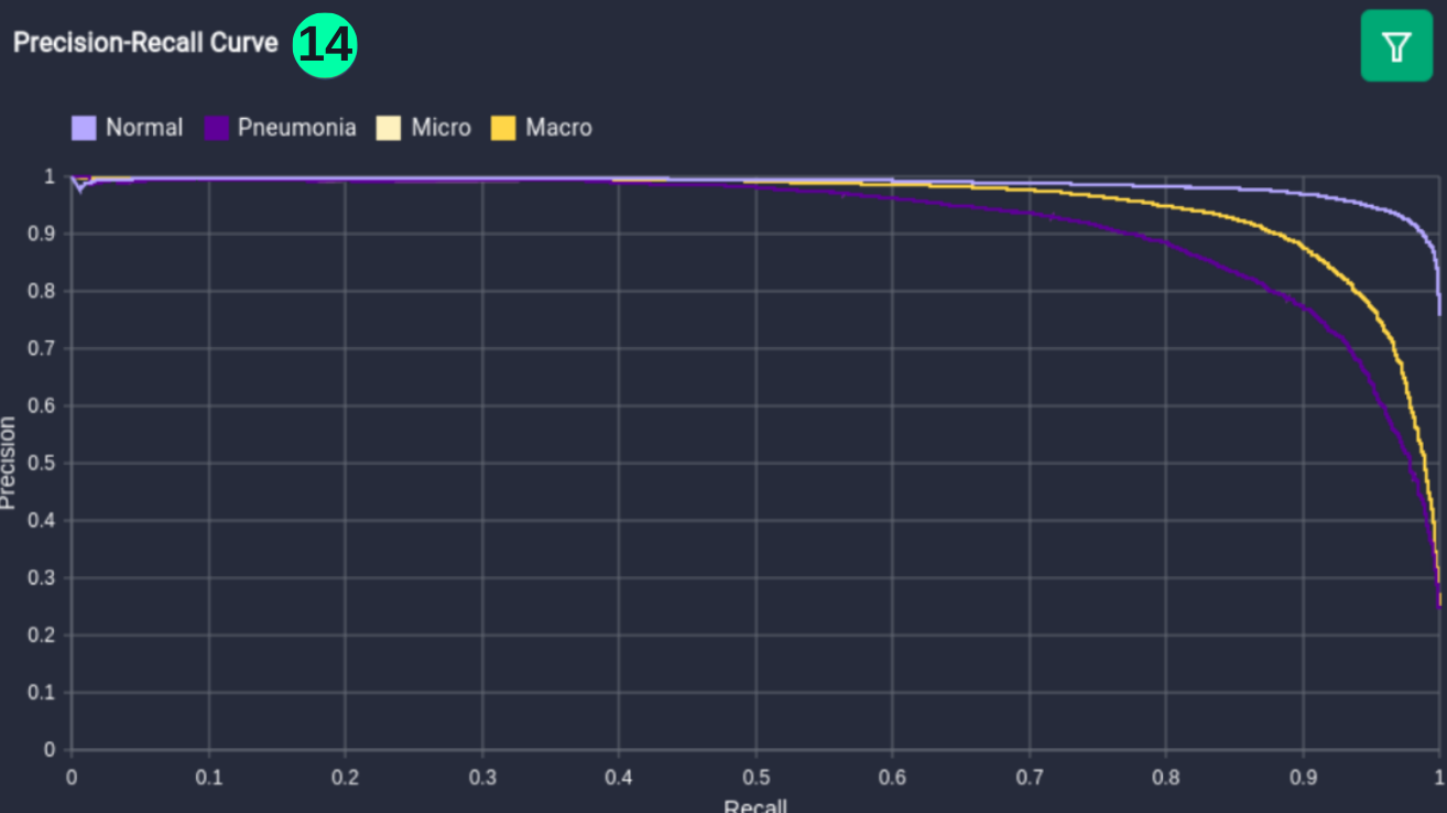
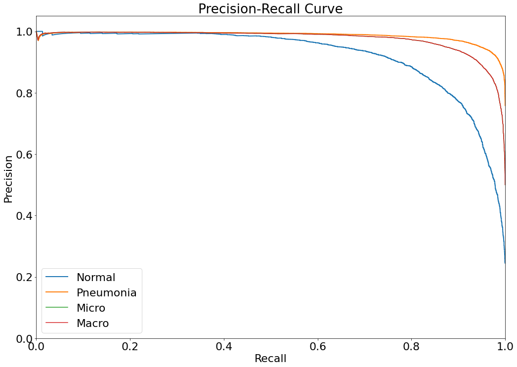
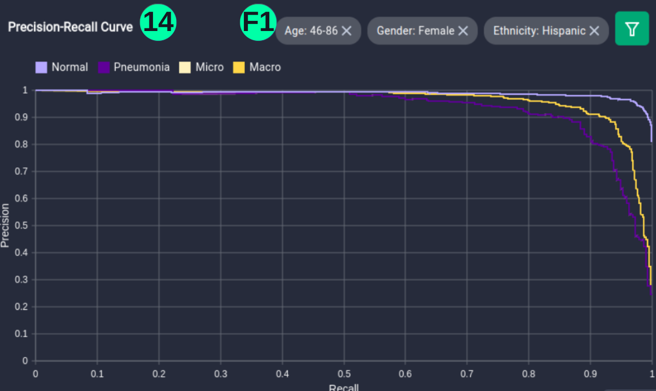
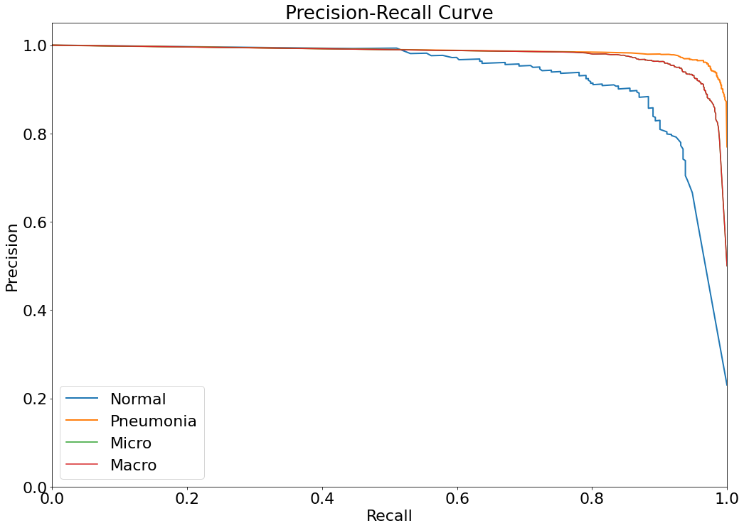
Precision-Recall Curve

• The Precision-Recall curve is constructed by calculating and plotting the precision against the recall for a single classifier at a variety of thresholds values. (Reference: https://analyticsindiamag.com/complete-guide-to-understanding-precision-and-recall-curves/)

(14) Results from the Snapshot of the platform can be compared with the documented results here:

from sklearn.metrics import precision_recall_curve
plt.figure(figsize=(17, 12))    

precision = dict()
recall = dict()
for i in range(n_classes):
    precision[i], recall[i], _ = precision_recall_curve(GT_binarized[:, i],
                                                        Probs[:, i])
    plt.plot(recall[i], precision[i], lw=2,label='{0}'
                                   ''.format(labels[i]))
    
    
precision["micro"], recall["micro"], _ = precision_recall_curve(GT_binarized.ravel(), Probs.ravel())
precision["macro"], recall["macro"] = precision["micro"], recall["micro"]
plt.plot(recall["micro"], precision["micro"],
         label='Micro')

plt.plot(recall["macro"], precision["macro"],
         label='Macro')
       
plt.xlim([0.0, 1.0])
plt.ylim([0.0, 1.05])  
plt.xlabel("Recall")
plt.ylabel("Precision")
plt.legend(loc="best")
plt.title("Precision-Recall Curve")
plt.show()

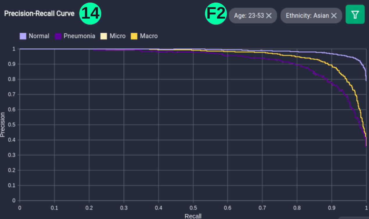
- The dataset and predictions can be filtered with metadata elements using the filter button, involving Age, Gender, and Ethnicity of the person, and Precision-Recall curves can be visualized for this setting.

(14)(F1) Filters and the resulting graph can be seen from the Snapshot of the platform and compared with the documented results here:

plt.figure(figsize=(17, 12))    

precision = dict()
recall = dict()
for i in range(n_classes):
    precision[i], recall[i], _ = precision_recall_curve(GT_F1_binarized[:,i], Probs_F1_np[:,i])
    plt.plot(recall[i], precision[i], lw=2,label='{0}'
                                   ''.format(labels[i]))
    
    
precision["micro"], recall["micro"], _ = precision_recall_curve(GT_F1_binarized.ravel(), Probs_F1_np.ravel())
precision["macro"], recall["macro"] = precision["micro"], recall["micro"]
plt.plot(recall["micro"], precision["micro"],
         label='Micro')

plt.plot(recall["macro"], precision["macro"],
         label='Macro')
       
plt.xlim([0.0, 1.0])
plt.ylim([0.0, 1.05])  
plt.xlabel("Recall")
plt.ylabel("Precision")
plt.legend(loc="best")
plt.title("Precision-Recall Curve")
plt.show()

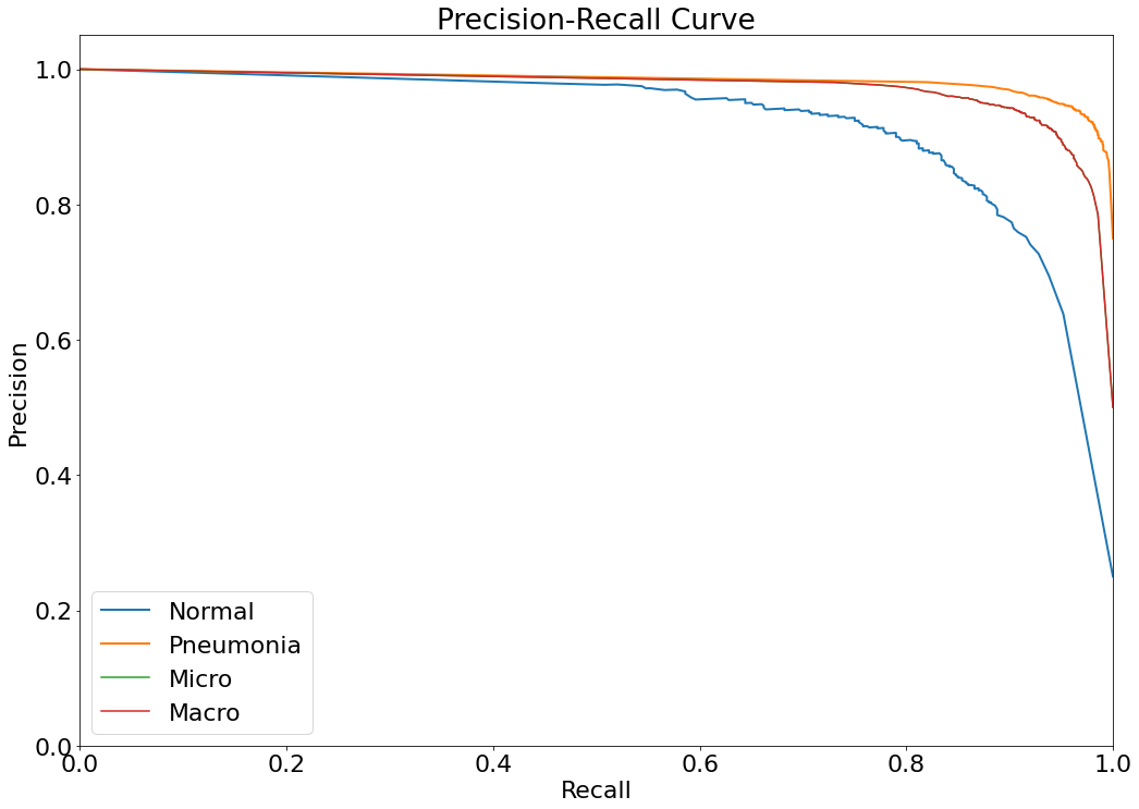
(14)(F2) Filters and the resulting graph can be seen from the Snapshot of the platform and compared with the documented results here:

plt.figure(figsize=(17, 12))    

precision = dict()
recall = dict()
for i in range(n_classes):
    precision[i], recall[i], _ = precision_recall_curve(GT_F2_binarized[:,i], Probs_F2_np[:,i])
    plt.plot(recall[i], precision[i], lw=2,label='{0}'
                                   ''.format(labels[i]))
    
    
precision["micro"], recall["micro"], _ = precision_recall_curve(GT_F2_binarized.ravel(), Probs_F2_np.ravel())
precision["macro"], recall["macro"] = precision["micro"], recall["micro"]
plt.plot(recall["micro"], precision["micro"],
         label='Micro')

plt.plot(recall["macro"], precision["macro"],
         label='Macro')
       
plt.xlim([0.0, 1.0])
plt.ylim([0.0, 1.05])  
plt.xlabel("Recall")
plt.ylabel("Precision")
plt.legend(loc="best")
plt.title("Precision-Recall Curve")
plt.show()

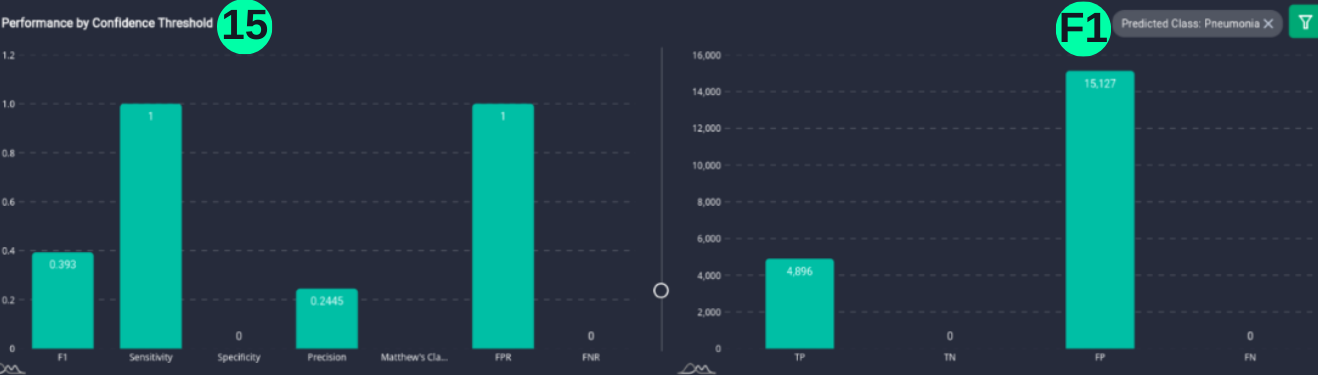
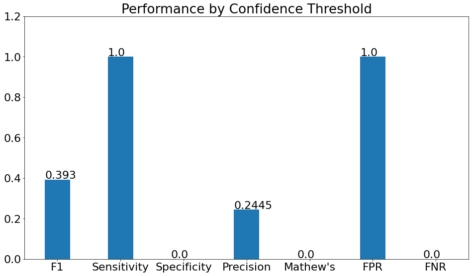
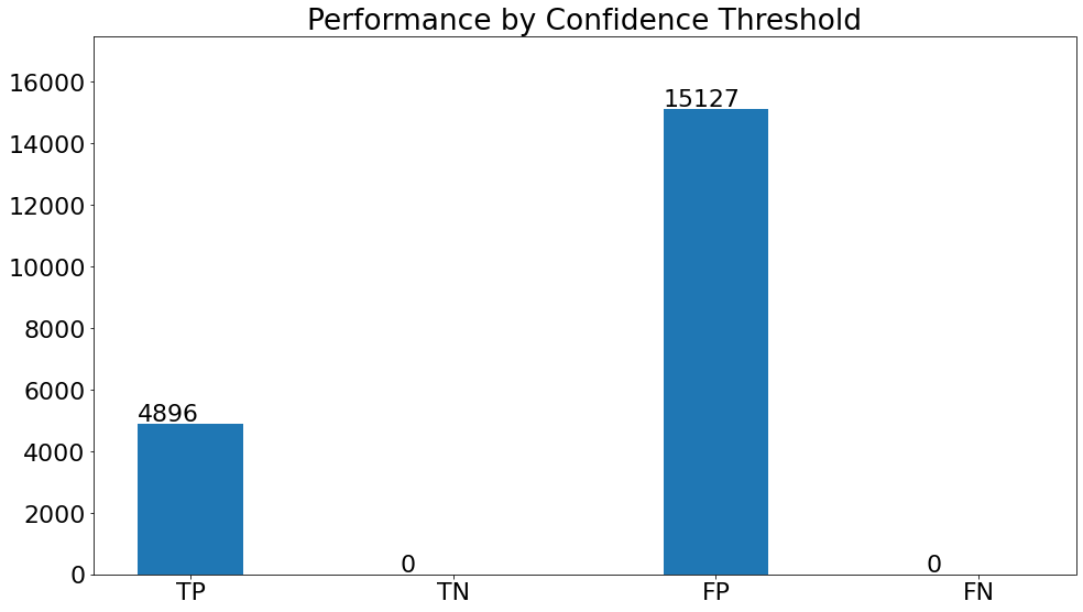
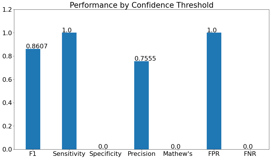
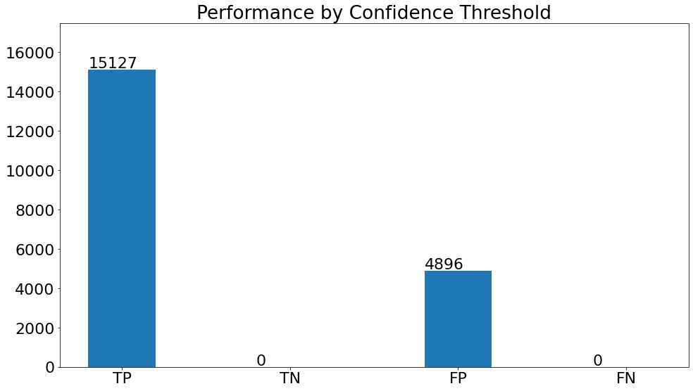
Performance by Confidence Threshold

• This chart shows the variation in the validation metrics by changing the prediction threshold through the vertical slider. The variation of results can be shown according to set filters.

(15)(F1) The resulting graph for the "Pneumonia" Class and Set Threshold of "0.2" can be seen from the Snapshot of the platform and compared with the documented results here:

target_class_list = ["Pneumonia"]
threshold = 0.2

for target_class in target_class_list:
    print(f"For {target_class}:" , "\n")
    
    ## Filter Class
    str_idx = 1 if target_class == "Pneumonia" else 0

    ## Threshold the probabilities
    target_class_confidence = Overall_df[f"Class_{str_idx}_Confidence"]
    target_class_threshold_indices = np.array(target_class_confidence>threshold)
    
    ## Get the thresholded prediction/ground truth
    thresholded_target_class_pred = np.ones(target_class_threshold_indices.sum())* class_mappings[target_class]
    GroundTruths_np_thresholded = GroundTruths_np[target_class_threshold_indices]
    GroundTruths_np_thresholded = (GroundTruths_np_thresholded == class_mappings[target_class])*1
    thresholded_target_class_pred = (thresholded_target_class_pred == class_mappings[target_class])*1
    f1_score_ = f1_score(GroundTruths_np_thresholded, thresholded_target_class_pred,average='binary' )
    sensitivity = recall_score(GroundTruths_np_thresholded, thresholded_target_class_pred, average='binary')
    TN, FP, FN, TP = confusion_matrix(GroundTruths_np_thresholded, thresholded_target_class_pred).ravel()
    specificity = TN/(TN+FP)
    precision = precision_score(GroundTruths_np_thresholded, thresholded_target_class_pred, average='binary')
    matthews_score = matthews_corrcoef(GroundTruths_np_thresholded, thresholded_target_class_pred)
    fnr = FN/(FN+TP)
    fpr = FP / (FP+TN)

plt.figure(figsize=(16, 9)) 
metricsss = ['F1','Sensitivity','Specificity','Precision',"Mathew's",'FPR','FNR',]
Count1 = [round(f1_score_,4),round(sensitivity,4),round(specificity,4),round(precision,4),round(matthews_score,4),
          round(fpr,4),round(fnr,4)]

bars = plt.bar(metricsss, height=Count1, width=.4)
xlocs, xlabs = plt.xticks()
xlocs=[i for i in metricsss]
xlabs=[i for i in metricsss]
plt.xticks(xlocs, xlabs)
  
for bar in bars:
    yval = bar.get_height()
    plt.text(bar.get_x(), yval + .005, yval)
plt.ylim([0,1.2]) 
plt.title('Performance by Confidence Threshold')
plt.show()


plt.figure(figsize=(16, 9)) 
tpfn = ['TP','TN','FP','FN']
Count2 = [TP, TN, FP, FN]

bars = plt.bar(tpfn, height=Count2, width=.4)
xlocs, xlabs = plt.xticks()
xlocs=[i for i in tpfn]
xlabs=[i for i in tpfn]
plt.xticks(xlocs, xlabs)
  
for bar in bars:
    yval = bar.get_height()
    plt.text(bar.get_x(), yval + 100, yval)
plt.ylim([0,17500]) 
plt.title('Performance by Confidence Threshold')
plt.show()

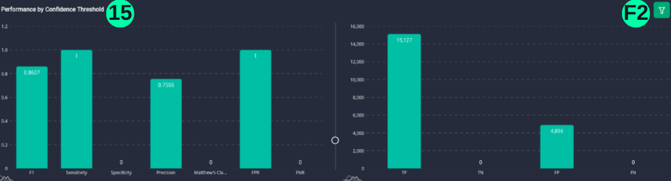
(15)(F2) The resulting graph for the "Normal" Class and Set Threshold of "0.2" can be seen from the Snapshot of the platform and compared with the documented results here:

target_class_list = ["Normal"]
threshold = 0.2

for target_class in target_class_list:
    print(f"For {target_class}:" , "\n")
    
    ## Filter Class
    str_idx = 1 if target_class == "Pneumonia" else 0

    ## Threshold the probabilities
    target_class_confidence = Overall_df[f"Class_{str_idx}_Confidence"]
    target_class_threshold_indices = np.array(target_class_confidence>threshold)
    
    ## Get the thresholded prediction/ground truth
    thresholded_target_class_pred = np.ones(target_class_threshold_indices.sum())* class_mappings[target_class]
    GroundTruths_np_thresholded = GroundTruths_np[target_class_threshold_indices]
    GroundTruths_np_thresholded = (GroundTruths_np_thresholded == class_mappings[target_class])*1
    thresholded_target_class_pred = (thresholded_target_class_pred == class_mappings[target_class])*1
    f1_score_ = f1_score(GroundTruths_np_thresholded, thresholded_target_class_pred,average='binary' )
    sensitivity = recall_score(GroundTruths_np_thresholded, thresholded_target_class_pred, average='binary')
    TN, FP, FN, TP = confusion_matrix(GroundTruths_np_thresholded, thresholded_target_class_pred).ravel()
    specificity = TN/(TN+FP)
    precision = precision_score(GroundTruths_np_thresholded, thresholded_target_class_pred, average='binary')
    matthews_score = matthews_corrcoef(GroundTruths_np_thresholded, thresholded_target_class_pred)
    fnr = FN/(FN+TP)
    fpr = FP / (FP+TN)


plt.figure(figsize=(16, 9)) 
metricsss = ['F1','Sensitivity','Specificity','Precision',"Mathew's",'FPR','FNR',]
Count1 = [round(f1_score_,4),round(sensitivity,4),round(specificity,4),round(precision,4),round(matthews_score,4),
          round(fpr,4),round(fnr,4)]

bars = plt.bar(metricsss, height=Count1, width=.4)
xlocs, xlabs = plt.xticks()
xlocs=[i for i in metricsss]
xlabs=[i for i in metricsss]
plt.xticks(xlocs, xlabs)
  
for bar in bars:
    yval = bar.get_height()
    plt.text(bar.get_x(), yval + .005, yval)
plt.ylim([0,1.2]) 
plt.title('Performance by Confidence Threshold')
plt.show()


plt.figure(figsize=(16, 9)) 
tpfn = ['TP','TN','FP','FN']
Count2 = [TP, TN, FP, FN]

bars = plt.bar(tpfn, height=Count2, width=.4)
xlocs, xlabs = plt.xticks()
xlocs=[i for i in tpfn]
xlabs=[i for i in tpfn]
plt.xticks(xlocs, xlabs)
  
for bar in bars:
    yval = bar.get_height()
    plt.text(bar.get_x(), yval + 100, yval)
plt.ylim([0,17500]) 
plt.title('Performance by Confidence Threshold')
plt.show()    

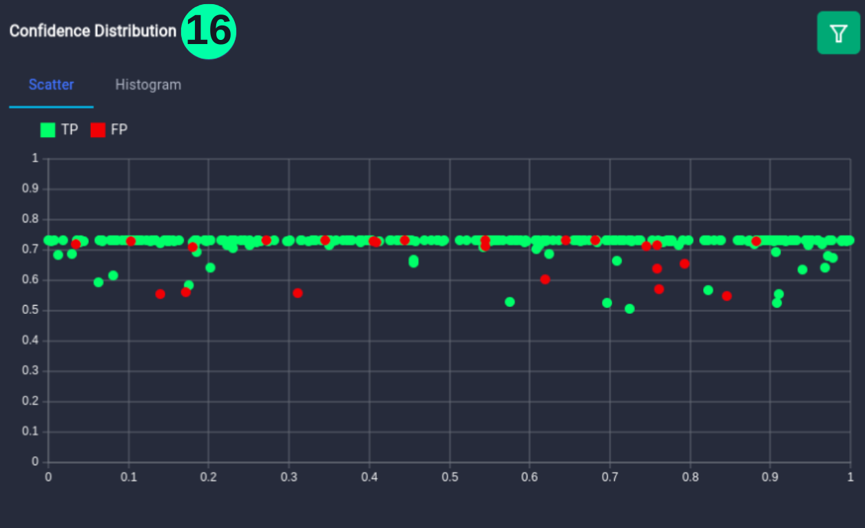
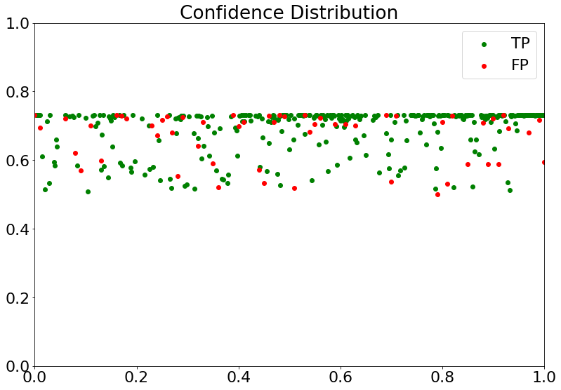
Confidence Distribution

• Represents the confidence value of every prediction, colored green for True Positive (TP) and red for False Positive (FP).

(16) Results from the Snapshot of the platform can be compared with the documented results here:

TP = []
FP = []
index = []     
index2 =[]
for i in range(np.size(GroundTruths_np)):
    if GroundTruths_np[i]==Predictions_np[i]:
        if GroundTruths_np[i] == 0:
            TP.append(Class_2_Confidence_np[i])
            index.append(i/500)
        else:
            TP.append(Class_1_Confidence_np[i])
            index.append(i/500)
    
for i in range(np.size(GroundTruths_np)):
    if GroundTruths_np[i] != Predictions_np[i]:
        if Predictions_np[i] == 1:
            FP.append(Class_1_Confidence_np[i])
            index2.append(i/100)

plt.figure(figsize=(13, 9)) 
plt.xlim([0.0, 1.0])
plt.ylim([0.0, 1.0]) 
plt.scatter(index, TP, class="gesundWord")
plt.scatter(index2, FP, color='red')
plt.legend(["TP" , "FP"])
plt.title("Confidence Distribution")
plt.show()

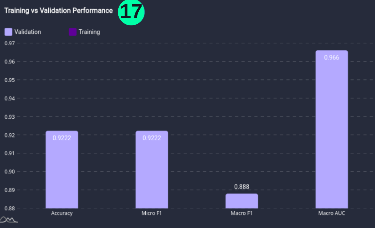
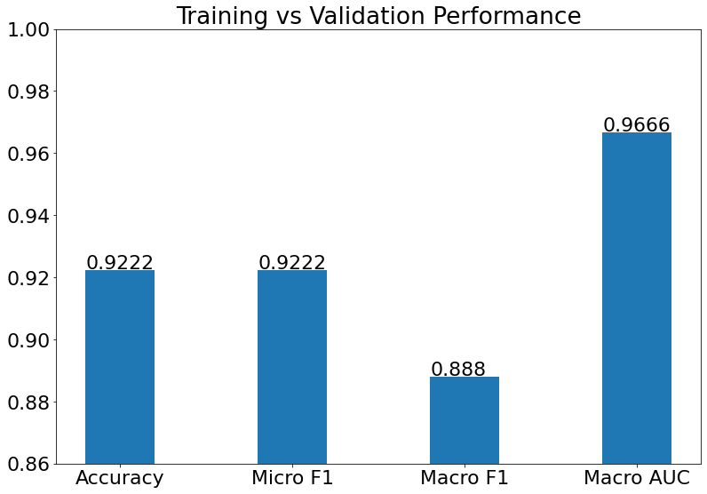
Training vs Validation Performance

• Training vs Validation Performance is the performance of the model on the training and validation datasets.

(17) Results from the Snapshot of the platform can be compared with the documented results here:

plt.figure(figsize=(13, 9)) 
Metric = ['Accuracy','Micro F1','Macro F1','Macro AUC']
Score = [round(Acc,4),round(Micro_F1,4),round(Macro_F1,4),round(roc1,4)]

bars = plt.bar(Metric, height=Score, width=.4)
xlocs, xlabs = plt.xticks()
xlocs=[i for i in Metric]
xlabs=[i for i in Metric]
plt.xticks(xlocs, xlabs)
  
for bar in bars:
    yval = bar.get_height()
    plt.text(bar.get_x(), yval + .0005, yval)
plt.ylim([0.86, 1.00]) 
plt.title('Training vs Validation Performance')
plt.show()

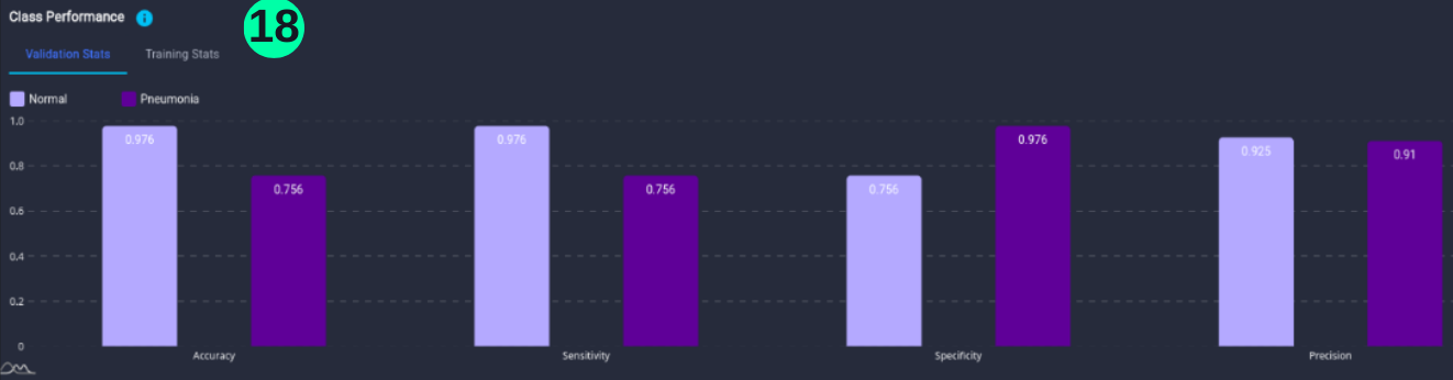
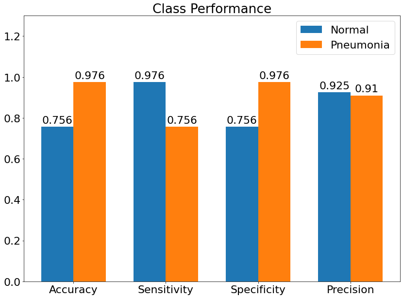
Class Performance

• Class Performance is the performance of the model for each class.

(18) Results from the Snapshot of the platform can be compared with the documented results here:

plt.rcParams["figure.figsize"] = (12,9)

labels = ['Accuracy', 'Sensitivity', 'Specificity', 'Precision']
Normal = [round(Acc1,3), round(Recall2,3), round(Recall1,3), round(Precision2,3)]
Pneumonia = [round(Acc2,3),round(Recall1,3), round(Recall2,3), round(Precision1,3)]


x = np.arange(len(labels))  # the label locations
width = 0.35  # the width of the bars

fig, ax = plt.subplots()
rects1 = ax.bar(x - width/2, Normal, width, label='Normal')
rects2 = ax.bar(x + width/2, Pneumonia, width, label='Pneumonia')

# Add some text for labels, title and custom x-axis tick labels, etc.
ax.set_title('Class Performance')
ax.set_xticks(x, labels)
ax.legend()

ax.bar_label(rects1, padding=3)
ax.bar_label(rects2, padding=3)

fig.tight_layout()
plt.ylim([0, 1.3]) 
plt.show()

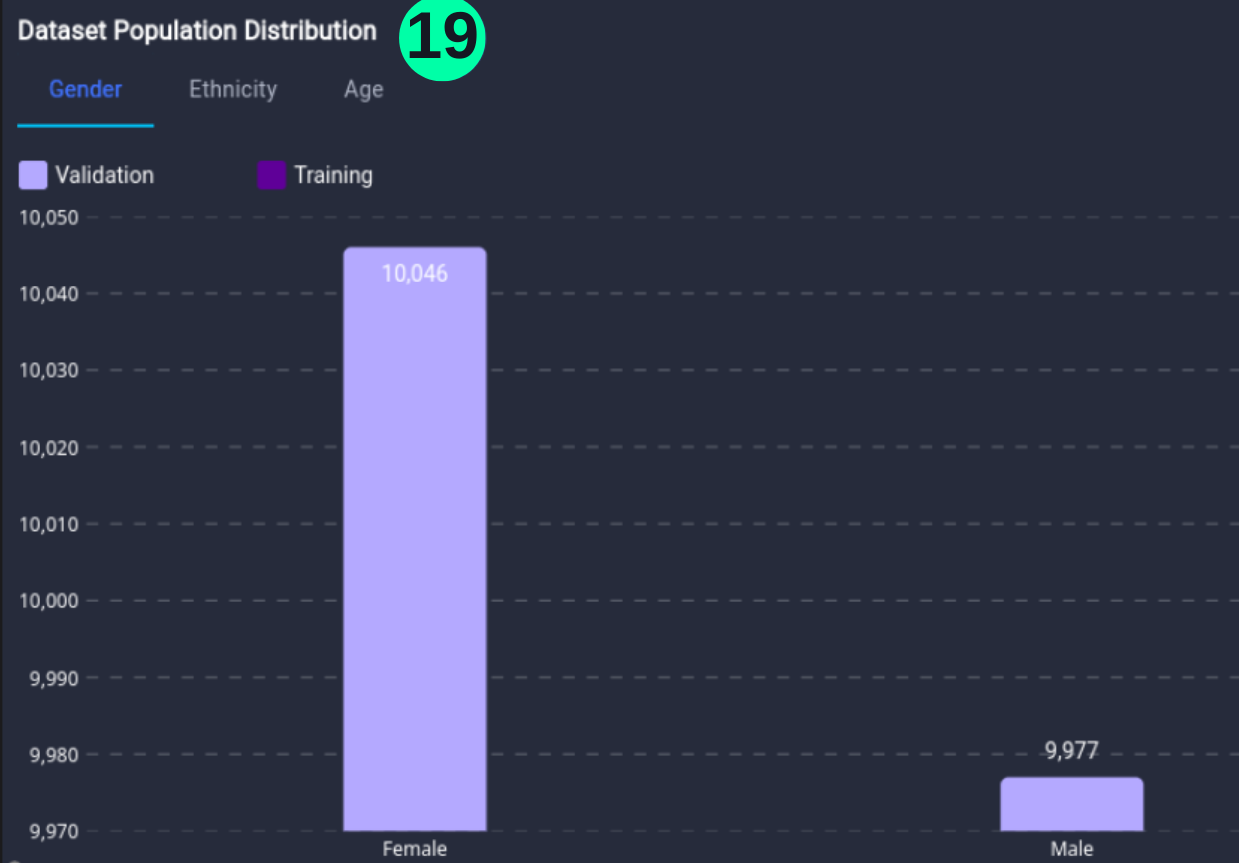
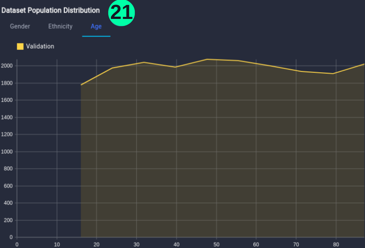
Dataset Population Distribution

• Chart to visualize the distribution in the dataset according to Metadata i.e. the person's Age, Ethnicity, and Age.

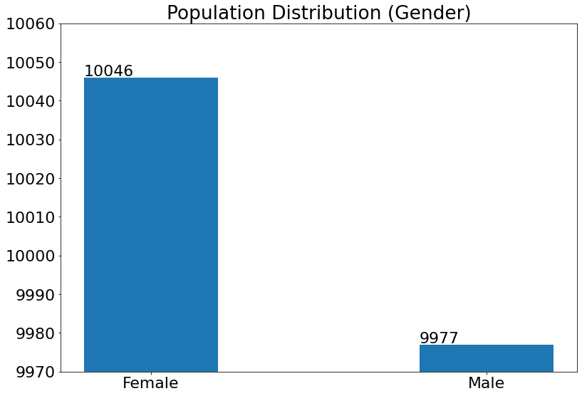
For Gender:

(19) Results from the Snapshot of the platform can be compared with the documented results here:

Male_num = len(Overall_df.loc[(Overall_df['Gender'] == 'Male')])
Female_num = len(Overall_df.loc[(Overall_df['Gender'] == 'Female')])


plt.figure(figsize=(13, 9)) 
Gender = ['Female','Male']
Count = [Female_num,Male_num]

bars = plt.bar(Gender, height=Count, width=.4)
xlocs, xlabs = plt.xticks()
xlocs=[i for i in Gender]
xlabs=[i for i in Gender]
plt.xticks(xlocs, xlabs)
  
for bar in bars:
    yval = bar.get_height()
    plt.text(bar.get_x(), yval + .5, yval)
plt.ylim([9970,10060]) 
plt.title('Population Distribution (Gender)')
plt.show()

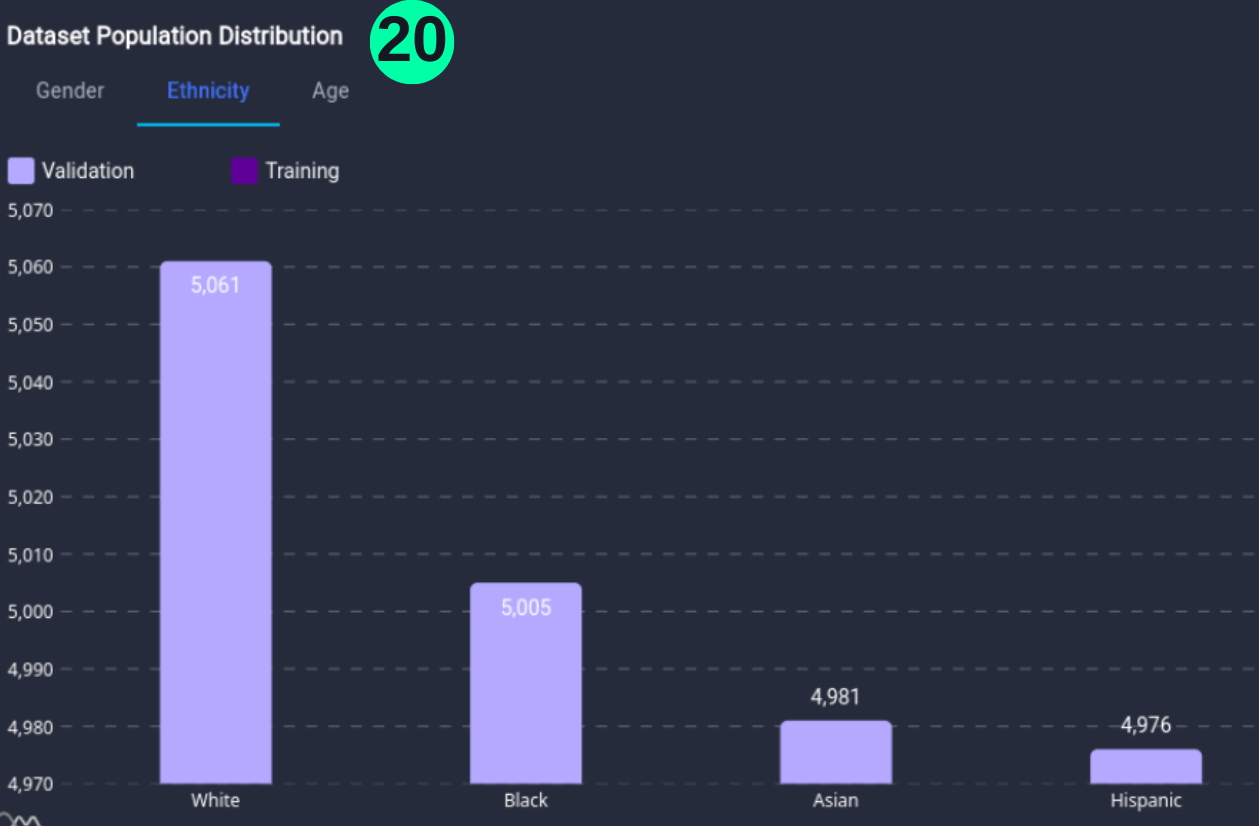
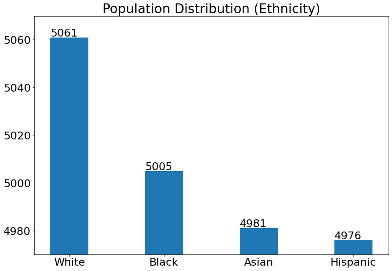
For Ethnicity:

(20) Results from the Snapshot of the platform can be compared with the documented results here:

White_num = len(Overall_df.loc[(Overall_df['Ethnicity'] == 'White')])
Black_num = len(Overall_df.loc[(Overall_df['Ethnicity'] == 'Black')])
Asian_num = len(Overall_df.loc[(Overall_df['Ethnicity'] == 'Asian')])
Hispanic_num = len(Overall_df.loc[(Overall_df['Ethnicity'] == 'Hispanic')])

plt.figure(figsize=(13, 9)) 
Eth = ['White','Black','Asian','Hispanic']
Count = [White_num,Black_num,Asian_num,Hispanic_num]

bars = plt.bar(Eth, height=Count, width=.4)
xlocs, xlabs = plt.xticks()
xlocs=[i for i in Eth]
xlabs=[i for i in Eth]
plt.xticks(xlocs, xlabs)
  
for bar in bars:
    yval = bar.get_height()
    plt.text(bar.get_x(), yval + .5, yval)
plt.ylim([4970,5070]) 
plt.title('Population Distribution (Ethnicity)')
plt.show()

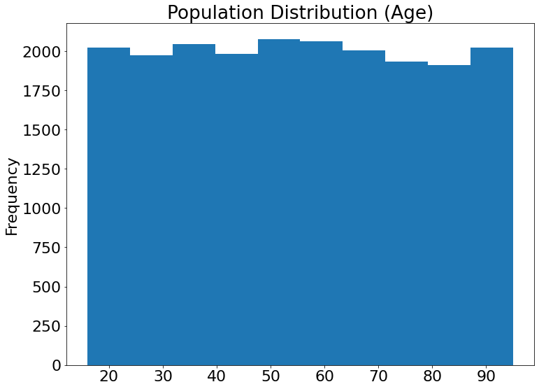
For Age:

(21) Results from the Snapshot of the platform can be compared with the documented results here:

df1 = Overall_df.sort_values(by=['Age'])
df2 = pd.DataFrame().assign(Age = df1['Age'])
df3 =df2.sort_values(by='Age', ignore_index=True)
df3['Count'] = df3['Age'].map(df3['Age'].value_counts())
df3["Age"].plot(kind = 'hist',title='Population Distribution (Age)')

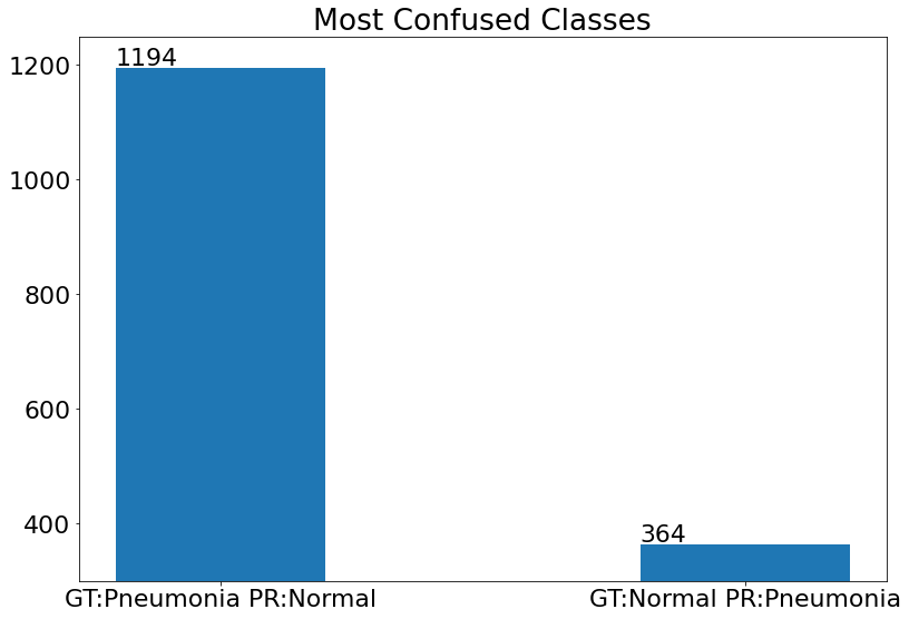
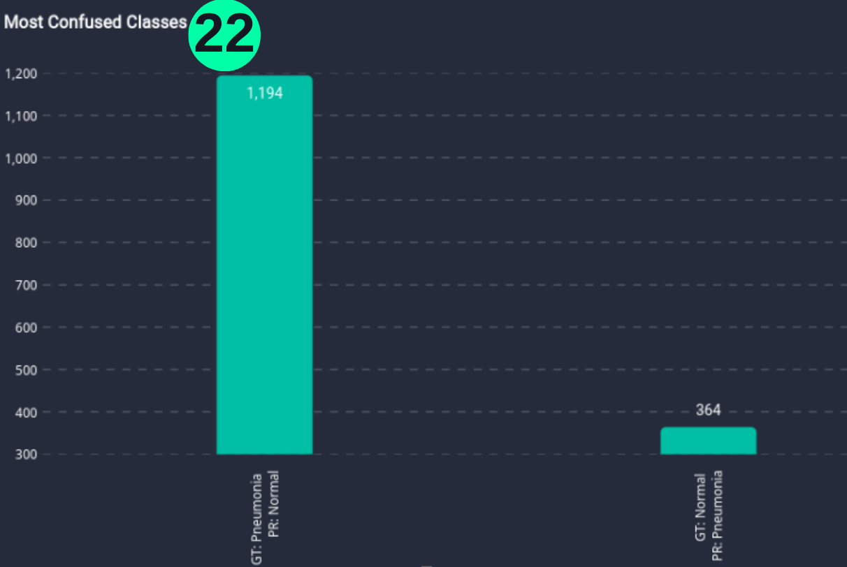
Most Confused Classes

• Bar chart that explains the model's most confused classes.

(22) Results from the Snapshot of the platform can be compared with the documented results here:

plt.figure(figsize=(13, 9)) 
con = ['GT:Pneumonia PR:Normal','GT:Normal PR:Pneumonia']
Count = [FP2,FN2]

bars = plt.bar(con, height=Count, width=.4)
xlocs, xlabs = plt.xticks()
xlocs=[i for i in con]
xlabs=[i for i in con]
plt.xticks(xlocs, xlabs)
  
for bar in bars:
    yval = bar.get_height()
    plt.text(bar.get_x(), yval + 5, yval)
plt.ylim([300,1250]) 
plt.title('Most Confused Classes')
plt.show()